TL;DR

To describe one fraction, use a binomial. To describe your uncertainty about that fraction, use a beta. To describe a collection of related fractions, use a beta-binomial.

What’s the Right Way to Aggregate Fractions?

Imagine you’re in the middle of building something awesome, when you realize that you have a problem that sounds something like one of the following:

A reddit user has submitted a bunch of URLs. Each one has a different number of upvotes and downvotes. How good is this user?

They’ve just posted a new link. That link has one downvote. Do we show it to more people or let it die in obscurity?
An author on a news site has written a collection of articles, each with a different bounce rate. How effective is this writer at driving traffic to the rest of the site?

They’ve just posted a new article. Should we promote it?
A supplier produces a bunch of different products sold on your website. Each one has a different average star rating. How good are the products from this supplier?

They’ve just added a new product to their catalog. How should we rank this against items from other suppliers that already have ratings?

In all of these situations you’ve measured a whole bunch of fractions. You think that these fractions have something in common because the same entity is responsible for them, but you don’t think they are exactly the same. Even if you had an infinite amount of data, each item would still be different. The collection of things made by each user or author or supplier has a range of quality. How can we accurately describe this range? Once we’ve described it, how can we use this to guess the quality of the next thing this entity does?

Henceforth, I’m going to use the reddit example, but it applies to a ton of different situations. For instance, It is one of the most common statistical problems we encounter in search.

What’s Wrong with Something Simple?

We have a whole bunch of fractions. We want to summarize them in some way to describe each user. Aggregating them seems like the reasonable thing to do. How could we aggregate them?

Add all the numerators, add all the denominators, and divide?

Consider the case of a notorious spammer who gets downvoted every time he posts, except one time he gets lucky, and a post takes off. The average for this spammer would be high, even though almost all of his submissions are horrible.

Count each fraction as 1 and take the average of all of them?

Consider a user who regularly makes fantastic comments with lots of upvotes, but periodically gets into a flame war with a single user who downvotes every comment in the thread. Those comments with a single downvote would get the same weight as the great comments, even though they represent the opinions of a very small number of people.
Weight each fraction by its denominator (equivalent to #1) except cap the denominator at something reasonable so that the average isn’t dominated by a single fraction?

Now we’re getting somewhere. This is how the system we’re going to derive behaves. It figures out the cap automatically, and it’s not quite a cap, but if you want to implement the simplest approximation of the Right Way™, weight each fraction by $n / (n + c)$ (where $c$ is some arbitrary constant, and $n$ is the denominator) and call it a day. However, the Right Way™ is much power powerful than this so read on!

Reddit’s karma system currently accumulates the total number of upvotes minus downvotes. This is good for encouraging users to post, but not at predicting the quality of a user’s posts. We can do better.

Dealing with One Fraction: The Binomial

Before we work on inferring something from a collection of fractions, let’s figure out how to deal with one fraction.

Any time you are measuring a fraction and describing it as a probability, you are talking about a binomial distribution. If you test something $n$ times and have $k$ positive results, then the distribution of outcomes follows

$\displaystyle P(k|p, n)=\text{Binomial}(k|p,n) =\binom{n}{k}p^k(1-p)^{n-k}$

$upvote-fraction-small$ In the reddit example, $n$ would be the total number of votes on an item, and $k$ would be the number of upvotes. If we want to describe the quality of a post, really we want to know the value of $p$ for this post. That is, if we collect an infinite number of votes on an item, what fraction of them will be upvotes?

What can we conclude about $p$ from the information we have about a post so far? Let’s use Bayes’ Rule to change the conditioning.

$\displaystyle P(k|p,n) = \text{Binomial}(k|p,n)$

$\displaystyle P(p|k,n) = \frac{\text{Binomial}(k|p,n)P(p)}{P(k|n)}$

$P(k|n) =\int_pP(k|p,n)$ . It is integrated over all of the possible values of $p$ so it doesn’t depend on any particular value of $p$ (just a normalization.) For simplicity right now we’ll assume that our prior of $P(p)$ is flat. This means that if we temporarily switch from $=$ to $\propto$ we can drop both terms. A common trick when working with complicated distributions is to say “We know this integrates to 1, so let’s drop all of the normalization terms and figure out what they have to be once we know the form of the distribution.”

$\displaystyle P(p|k,n) \propto \text{Binomial}(k|p,n)$

$\displaystyle P(p|k, n) \propto \binom{n}{k}p^k(1-p)^{n-k}$

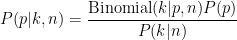
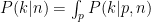
The difference between this formula and the one we started with is that $p$ is now the variable, and the other terms are fixed. This makes it a different distribution, the beta distribution, because it is now a continuous distribution over $p$ instead of a discrete distribution over $k$ .

We’ll get back to the beta distribution in a second. For now we’re just concerned with $p$ . For the data we’ve observed so far, what’s the most likely value of $p$ ? Let’s maximize its log with respect to $p$ . (Since log is monotonic, maximizing the log of a positive function is the same as maximizing the function, and it almost always makes for easier math.)

$\displaystyle \log P(p|k,n) = C + \log \binom{n}{k}p^k(1-p)^{(n-k)}$

$\displaystyle \log P(p|k,n) = C' + \log p^k + \log (1-p)^{(n-k)}$

$\displaystyle \frac{d\log P(p|k,n)}{dp} = \frac{k}{p} - \frac{n-k}{1-p}$

$\displaystyle 0 = \frac{k}{p} - \frac{n-k}{1-p}$

$\displaystyle \frac{p}{1-p} = \frac{k}{n-k}$

$\displaystyle p = \frac{k}{n}$

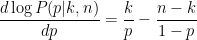
Wow, that’s about as intuitive as it gets. When you estimate the probability of an event as the fraction of times it happened ( $k/n$ ), you are really choosing the most likely parameter of the binomial distribution, even though you probably didn’t know it.

Now we know how to deal with one fraction, and how to guess its $p$ . Each fraction for a user will have a different $p$ , but we think they are still related somehow. What describes the relationship between the different $p$ ‘s?

Representing Uncertainty about a Fraction: The Beta Distribution

The beta distribution is a smooth distribution over the interval $[0,1]$ . It looks like a bell curve, but the way a bell curve would look like if you squished it into a box. $\alpha$ and $\beta$ are its two parameters. $\alpha/(\alpha + \beta)$ describes the center of the distribution, and $\alpha + \beta$ describes how tight it is.

$\displaystyle P(p|\alpha, \beta)=\text{Beta}(p | \alpha, \beta)=\frac{\Gamma(\alpha+\beta)}{\Gamma(\alpha)\Gamma(\beta)}p^{\alpha-1}(1-p)^{\beta-1}$

Notice that the beta distribution has the same form as the binomial distribution, but with $\alpha - 1$ and $\beta - 1$ exchanged for $k$ and $n-k$ , continuous versions of factorial (gamma), and $p$ as the random variable instead of a parameter. This fact is why the beta distribution is important.

Beta distributions with the same variance

When we assume we have no information about the distribution of $p$ , then observe samples from the binomial, our uncertainty about $p$ follows a beta distribution. What happens if instead of a flat prior we assume a beta distribution for the prior of $p$ ? The combined distribution of $k$ and $p$ becomes:

$P(x, p|n, \alpha, \beta) = \text{Binom}(x | p, n) \text{Beta}(p | \alpha, \beta)$

$P(x, p|n, \alpha, \beta) = \binom{n}{k}p^k(1-p)^{n-k}\frac{\Gamma(\alpha+\beta)}{\Gamma(\alpha)\Gamma(\beta)}p^{\alpha-1}(1-p)^{\beta-1}$

As above, we’ll change the conditioning by noting that the prior probability $P(x)$ doesn’t depend on the individual value of $p$ and dropping the normalization terms.

$P(p|x, n, \alpha, \beta) \propto p^k(1-p)^{n-k}p^{\alpha-1}(1-p)^{\beta-1}$

$P(p|x, n, \alpha, \beta) \propto p^{k + \alpha -1}(1-p)^{n-k + \beta-1}$

From the knowledge that this is a probability distribution and thus integrates to 1, we can put in gamma terms that we know will normalize the distribution and change $\propto$ back to $=$ .

$P(p|x, n, \alpha, \beta) =\frac{\Gamma(n + \alpha + \beta)}{\Gamma(k +\alpha)\Gamma(n-k+\beta)} p^{k + \alpha -1}(1-p)^{n-k + \beta-1}$

Look how nicely that collapsed! We end up with another beta distribution for $p$ . For this reason, the Beta distribution is the “Conjugate Prior” of the binomial. If your prior knowledge about $p$ is a beta, your posterior after observing some binomial samples is also a beta.

This makes the beta distribution an extremely convenient choice for representing the range of quality of each user! If we express that range of quality as a beta distribution, then we can easily make good guesses about the quality of a post no matter how many votes it has by maximizing the above formula! Our best guess as derived in the previous section becomes

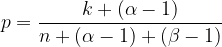
$\displaystyle p = \frac{k + (\alpha - 1)}{n + (\alpha - 1) + (\beta - 1)}$

So if we have a beta distribution for each user, doing the right thing to rank their posts is now exceedingly easy. Notice how the $\alpha - 1$ and $\beta - 1$ are effectively fictitious counts, as if we observed some additional data. These are called “pseudocounts” and they crop up frequently in the math of combining priors with evidence. Later on we’re going to work out in great detail how to fit the beta distribution for each user, but despite sounding complicated, it finally has a very simple interpretation. Each user’s posts will start out their life with $\alpha -1$ upvotes and $\beta - 1$ downvotes, determined by the history of votes they’ve gotten on their other posts.

To figure out the beta distribution for each user, somehow we have to infer it from the collection of numerators and denominators of their posts. We’ll do this using the combined distribution.

$P(x_i,p_i|n_i,\alpha,\beta)=\text{Binom}(x_i|p_i, n_i) \text{Beta}(p_i | a, b)$

This combined distribution of binomial samples generated from a beta is called the Beta-Binomial.

How do we fit a Beta-Binomial?

The joint probability of the data and the values of $p$ takes the following form.

$P(x_i, p_i|n_i, \alpha, \beta) = \text{Binom}(x_i | p_i, n_i) \text{Beta}(p_i | a, b)$

If we knew the values of $p$ , we could maximize this w.r.t. $\alpha$ and $\beta$ , but we don’t know the values of $p$ . If we knew the values of $\alpha$ and $\beta$ we could maximize this w.r.t. $p_i$ and find the values of $p$ for each binomial (as we derived above), but we don’t know the values of $\alpha$ and $\beta$ .

This is a perfect opportunity to use Expectation Maximization, an optimization technique that lets us alternate between fitting $p$ and fitting $\alpha$ and $\beta$ , and converges to a locally optimal fit. Instead of integrating out $p_i$ and maximizing the resulting log likelihood, we’re iteratively maximizing the average value of the log likelihood under our current guess of the distribution of $p_i$ . (Integrating out $p_i$ is possible, but doing it this way instead has other benefits that I’ll mention later.)

Using the “Soft EM” version of the algorithm, we’ll be iteratively maximizing

$\displaystyle \sum_i\text{E}_{p_i|k_i,n_i,\alpha,\beta}[\log P(k_i,p_i|n_i,\alpha',\beta')]$

where $\alpha'$ and $\beta'$ are the values we are fitting, and $\alpha$ and $\beta$ are the values from the previous round. That’s a mouthful of an expression if you aren’t familiar with EM. What’s going on here?

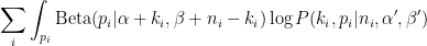
As we discussed above, from a binomial observation ( $n, k$ ) and a beta distribution prior ( $\alpha$ , $\beta$ ) we can come up with a beta distribution for the value of $p$ . Let’s rewrite the expectation.

$\displaystyle \sum_i\int_{p_i}\text{Beta}(p_i|\alpha + k_i, \beta + n_i-k_i)\log P(k_i,p_i|n_i,\alpha',\beta')$

$\displaystyle \sum_i\int_{p_i}\text{Beta}(p_i|\alpha + k_i, \beta + n_i-k_i)\left[\log \text{Binom}(x_i | p_i, n_i) +\log\text{Beta}(p_i | \alpha', \beta')\right]$

The first term is a data dependent constant that doesn’t depend on $\alpha'$ and $\beta'$ so we can drop it from the optimization.

$\displaystyle \sum_i\int_{p_i}\text{Beta}(p_i|\alpha+k_i,\beta+n_i-k_i)\log\text{Beta}(p_i|\alpha', \beta')$

If you know a bit about information theory, this term should look familiar. It’s the negative of the cross entropy between $\text{Beta}(p_i|\alpha+k_i,\beta+n_i-k_i)$ and $\text{Beta}(p_i|\alpha',\beta')$ . The distribution that minimizes the cross entropy will be the distribution itself. What this means intuitively is that we’re trying to pick $\alpha'$ and $\beta'$ to make the prior distribution as similar as possible to each posterior. Since each binomial is different, and thus has a different posterior, these are competing objectives. This is true of EM in general, but is particularly useful here. We’ll come back to this later.

Let’s break apart the Beta inside the log.

$\displaystyle \sum_i\int_{p_i}\text{Beta}(p_i|\alpha+k_i,\beta+n_i-k_i)\log \frac{\Gamma(\alpha'+\beta')}{\Gamma(\alpha')\Gamma(\beta')}p_i^{\alpha'} (1-p_i)^{\beta'}$

$\displaystyle N\log\frac{\Gamma(\alpha'+\beta')}{\Gamma(\alpha')\Gamma(\beta')}+\sum_i\int_{p_i}\text{Beta}(p_i|\alpha+k_i,\beta+n_i-k_i)\log p_i^{\alpha'} (1-p_i)^{\beta'}$

$\displaystyle N\log\frac{\Gamma(\alpha'+\beta')}{\Gamma(\alpha')\Gamma(\beta')}+\sum_i \alpha'E_{p_i}[\log p_i] + \beta'E_{p_i}[\log 1-p_i]$

These expectations of the log $p_i$ s are nicely derived on the wikipedia article for the beta distribution in the section on geometric means.

$\displaystyle N\log\frac{\Gamma(\alpha'+\beta')}{\Gamma(\alpha')\Gamma(\beta')}+\sum_i \alpha'[\psi(\alpha + k_i) - \psi(\alpha + \beta + n_i)] + \beta'[\psi(\beta+n_i-k_i) - \psi(\alpha + \beta + n_i)]$

Digamma (green) vs Log (grey) — Digamma (green), Log (grey)

$\psi(x)$ is the digamma function. In the limit, it behaves like $\log$ . The main difference between the two functions for our purposes is where x is small, close to 0, where $\psi(x)$ asymptotes much more quickly.

We’re ready to take some derivatives.

$\displaystyle \frac{\partial}{\partial \alpha'} = N(\psi(\alpha'+\beta') - \psi(\alpha')) +\sum_i\psi(\alpha + k_i) - \psi(\alpha + \beta + n_i)$

$\displaystyle \frac{\partial}{\partial \beta'} = N(\psi(\alpha'+\beta') - \psi(\beta')) +\sum_i\psi(\beta + n_i - k_i) - \psi(\alpha + \beta + n_i)$

When we set the partials to 0 and solve we get particularly beautiful relationships.

$\displaystyle\psi(\alpha')-\psi(\alpha'+\beta')=\frac{1}{N}\sum_i\psi(\alpha+k_i)-\psi(\alpha+\beta+n_i)$

$\displaystyle\psi(\beta')-\psi(\alpha'+\beta')=\frac{1}{N}\sum_i\psi(\beta+n_i-k_i)-\psi(\alpha+\beta+n_i)$

Unfortunately, solving this involves inverting the digamma function, which everyone seems to cite someone else for. I’m no exception. At this point I’ll refer you to Thomas Minka’s Estimating a Dirichlet Distribution where he works out both fixed point (slow) and newton iteration (fast) methods to solve for alpha and beta from this set of equations.

Without worrying about how to solve the terms on the left side, there’s a lot we can infer just looking at the expressions. Notice how the right side is just the average of a statistic collected over all of the samples. $\psi(x)$ behaves similar to $\log(x)$ when the values are large, which lets us simplify the equations for the purposes of understanding them. (Note that this simplification does not produce good numerical results, this digression is just to help understand what this is doing.)

$\displaystyle\log\left(\frac{\alpha'}{\alpha'+\beta'}\right)\approx\frac{1}{N}\sum_i\log\left(\frac{\alpha+k_i}{\alpha+\beta+n_i}\right)$

$\displaystyle\frac{\alpha'}{\alpha'+\beta'}\approx\left(\prod_i\frac{\alpha+k_i}{\alpha+\beta+n_i}\right)^{1/N}$

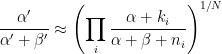
This tells us that the mean of the beta will be approximately the geometric mean of the smoothed values of $p$ for each binomial.

Let’s see what else we can figure out from these expressions. Consider the case where we’ve only measured 1 binomial sample, or all the binomials we’ve measured have the same $n$ and $k$ . In that case, the above equations are solved when $\alpha' = \alpha + k$ and $\beta' = \beta + n - k$ . Uh Oh. We’re running this iteratively, so both $\alpha$ and $\beta$ will diverge! What’s going on?

We didn’t include a prior for $\alpha$ and $\beta$ . We’re computing the maximum likelihood estimate, instead of the maximum a posteriori estimate. This means that the beta distribution can become as implausible as it wants to, so long as being implausible makes the data more likely. In this case, The beta distribution is turning into a delta function at the value of $p = k/n$ of the single binomial.

It’s doing the right thing, there isn’t a bug in our math. The delta function at that value is the maximum likelihood estimate when all of the binomials have the same $n$ and $k$ , but it’s clearly not what we want. Note too that this isn’t that much of an edge case. It can easily happen just by chance that all of our measured binomials are the same. It would be really bad if something so simple caused our code to run forever. We need either a prior, or some regularization.

Unfortunately, the beta distribution doesn’t have a convenient conjugate prior for us to use. Instead, let’s borrow the idea of “pseudocounts” from the binomial example. Our fit is expressed as a nice summary statistic averaged over all the binomials, and we showed how these represent cross entropies from the beta implied by each binomial. Let’s just add some fake ones. We’ll make up a beta with parameters $\alpha_\emptyset,\beta_\emptyset$ and give it a weight of $M$ relative to the other samples. Formally speaking, we’re adding a regularization term to the optimization that penalizes the beta’s divergence from an example beta as below.

$\displaystyle M\int_p\text{Beta}(p|\alpha_\emptyset,\beta_\emptyset)\log\text{Beta}(p|\alpha', \beta')+\sum_i\int_{p_i}\text{Beta}(p_i|\alpha+k_i,\beta+n_i-k_i)\log\text{Beta}(p_i|\alpha', \beta')$

These collapse nicely with our previous derivation, and turn into an equally convenient update rule. These terms force convergence, because they don’t update on each iteration.

$\displaystyle\psi(\alpha')-\psi(\alpha'+\beta')=\frac{1}{N+M}\left[M(\psi(\alpha_\emptyset)-\psi(\alpha_\emptyset+\beta_\emptyset))+\sum_i\psi(\alpha+k_i)-\psi(\alpha+\beta+n_i)\right]$

$\displaystyle\psi(\beta')-\psi(\alpha'+\beta')=\frac{1}{N+M}\left[(\psi(\beta_\emptyset)-\psi(\alpha_\emptyset+\beta_\emptyset))+\sum_i\psi(\beta+n_i-k_i)-\psi(\alpha+\beta+n_i)\right]$

The nice thing about these expressions is how intuitive they are. The difference of digammas may seem like a strange statistic, but finally you’re just averaging this function over all of your data, and then inverting it, just like you would average the values to compute a mean, or average the squared error to compute a variance.

Because this fitting process is expressed in terms of a summary statistic, we can easily implement a streaming version of this algorithm without any extra derivation. We buffer some data, fit the beta, then assume that these summary statistics of the difference of digammas are good enough to describe the points we’ve seen so far. We then discard those points, and keep only the current beta and a weight to reflect how much data we’ve already processed. This beta and weight posterior for our current fit become the prior for fitting the next buffer of data.

This is the advantage of this approach over integrating out $p_i$ and optimizing the likelihood function directly. It allows you to express an intuitive (approximate) prior for what the beta should look like, and permits a streaming version by describing your current fit in the same form as that approximate prior.

Simulated Data

In these charts I’ve simulated what real data might look like. In order to see the difference between them, there are two sets of plots, one for a beta-binomial, and one for a binomial.

Beta-Binomial

Sample $n$ from an exponential distribution with mean of 10.
Sample $p$ according to $\text{Beta}(p|\alpha=3,\beta=5)$ ,
Sample $k$ according to $\text{Binomial}(k|n,p)$

Binomial

Sample $n$ from an exponential distribution with mean of 10.
Sample $k$ according to $\text{Binomial}(k|n,p=3/(3+5))$ .

This is repeated 10,000 times. Both distributions have the same mean. The interesting pattern is in their spreads.

Scatter plot of n and k generated from a Beta-Binomial — n and k generated from a Beta-Binomial

Scatter plot of n and k generated from a Binomial — n and k generated from a Binomial

In the Beta-Binomial, the distribution continues to spread out as $n$ increases. In the binomial case, it stays tight around the slope of the mean.

Scatter plot of k/n and n generated from a Beta-Binomial — k/n and n generated from a Beta-Binomial

Scatter plot of k/n and n generated from a Binomial — k/n and n generated from a Binomial

As $n$ increases for a beta-binomial, the distribution of $k/n$ converges to the underlying beta. As $n$ increases for a binomial, $k/n$ converges to a point at $p$ .

Histogram of k/n generated from a Beta-Binomial

Histogram of k/n generated from a Binomial

These graphs are here solely to demonstrate the futility of understanding these distributions through a histogram. It is a very poor tool to understand a fraction computed over varying $n$ .

In the Real World

Worry more about what you are measuring than how you are measuring it. Getting the math right is a secondary consideration. You do this stuff after you have something simple that basically works. Break out the big guns to make it better, not in the hopes that it will make something work if the stupid version doesn’t already do pretty well.

For instance, In this article I’ve assumed that the ratio of upvotes to votes is the relevant measure of quality, but it may not be the best. It might be more interesting to measure the ratio of upvotes to impressions. Or maybe to measure independently the ratio of upvotes to all votes, and the ratio of all votes to impressions. There are many aspects of a user that you could (and should) attempt to describe in a complete system.

However, whatever aspect you are measuring, if you can express it as a fraction, chances are this is the technique you’ll want to use to describe it.

2 Comments

Brian says:

September 11, 2013 at 12:42 pm

This is a great post and exactly what I’m looking forward, although perhaps a bit complex. In the special case where all n_i are the same (although not relevant for you), the method of moments provides a simple technique as sketched out on wikipedia’s Beta-Binomial page. In fact, most articles I find discuss only the case where all n_i are the same. Do you know if its possible to do modified method of moments that would also solve this problem (even if it’s only a second order approximation)?

Thanks!

Ryan Moulton says:

September 11, 2013 at 12:57 pm

In the code that I’m preparing to release, I initialize using moment estimates with varying n, though it’s somewhat hacky. The mean is easy. The variance of the beta I approximate using the overdispersion. The wikipedia article relates the overdispersion parameter to the variance of the betabinomial http://en.wikipedia.org/wiki/Beta-binomial_distribution#Moments_and_properties. I estimate the overdispersion by inverting that function on each individual squared error, then guess the variance of that estimate hackily, and compute the weighted average over all the samples weighting by the inverse of the variance of each estimate.

It works well as an initialization, enough to speed things up 20x over what I was doing before, but it’s not something I’m terribly proud of. 🙂

How Karma Systems Should Work: The Beta-Binomial

TL;DR

What’s the Right Way to Aggregate Fractions?

What’s Wrong with Something Simple?

Dealing with One Fraction: The Binomial

Representing Uncertainty about a Fraction: The Beta Distribution

How do we fit a Beta-Binomial?

Simulated Data

In the Real World

2 Comments

Leave a comment Cancel reply

TL;DR

What’s the Right Way to Aggregate Fractions?

What’s Wrong with Something Simple?

Dealing with One Fraction: The Binomial

Representing Uncertainty about a Fraction: The Beta Distribution

How do we fit a Beta-Binomial?

Simulated Data

In the Real World

Share this:

Related

2 Comments

Leave a comment Cancel reply