
Clustering with a Key-Value Store
Let’s say you have a dataset you’d like to cluster. Let’s say you don’t want to write more than 5 lines of code. Let’s say that your only tool is a key-value store. (Why might you be in this position? Perhaps your dataset is really really (really) big and only simple things will scale. Maybe it’s in fact INFINITE and you’re clustering a stream. Maybe MapReduce is just a really big hammer. 🔨👷 Why you’d only want to write 5 lines of code is left as an exercise to the reader.)
At any rate, you would like to make clusters out of your data, but you only get to look at each item once in isolation. After looking at it you have to decide what cluster it should go to, at that moment, without looking at any other information, or any other items in your dataset. You only get one shot, do not throw it away! How can we accomplish this?
Ideally we want a magic function, 


Let’s say you have a function 
![\Pr\left[H(X) = H(Y)\right] = sim(X, Y)](https://s0.wp.com/latex.php?latex=%5CPr%5Cleft%5BH%28X%29+%3D+H%28Y%29%5Cright%5D+%3D+sim%28X%2C+Y%29&bg=%23ffffff&fg=%23000000&s=0&c=20201002)

// C++ code implementing each algorithm will be in a block like this one
// at the end of each section.
Building a Simple H(X): MinHash
Suppose you have two sets,

That’s nice, but isn’t comparable across different sizes of sets, so let’s normalize it by the union of the two sizes.

This is called the Jaccard Index, and is a common measure of set similarity. It has the nice property of being 0 when the sets are disjoint, and 1 when they are identical.
Suppose you have a uniform pseudo-random hash function 
![[0,1]](https://s0.wp.com/latex.php?latex=%5B0%2C1%5D&bg=%23ffffff&fg=%23000000&s=0&c=20201002)


Consider 
If you delete 


If you insert 


For our purposes, this means that
What is the probability that 
If an element produces the minimum hash in both sets on their own, it also produces the minimum hash in their union.


Look familiar? Presto, we now have a Locality Sensitive Hash for the Jaccard Index.

![\displaystyle P\left[H(X) = H(Y)\right] = \frac{|X\cap Y|}{|X\cup Y|}](https://s0.wp.com/latex.php?latex=%5Cdisplaystyle+P%5Cleft%5BH%28X%29+%3D+H%28Y%29%5Cright%5D%C2%A0+%3D+%5Cfrac%7B%7CX%5Ccap+Y%7C%7D%7B%7CX%5Ccup+Y%7C%7D+&bg=%23ffffff&fg=%23000000&s=0&c=20201002)
unsigned long long int MinHash(T X) {
  unsigned long long int min_hash = ULLONG_MAX;
  for (auto x : X) {
    min_hash = min(min_hash, Hash(x));
  }
  return min_hash;
}
Tuning Precision and Recall with Combinatorics
Now that we have a locality sensitive hash, we can use combinatorics to build something that looks a bit more like our magic function. We can concatenate (or sum) hashes to perform an “AND” operation. Let 


We can then output multiple hashes to perform an “OR” operation. If we output 

Using these two tools, we can apply a “sigmoid” function to our similarities, outputting 
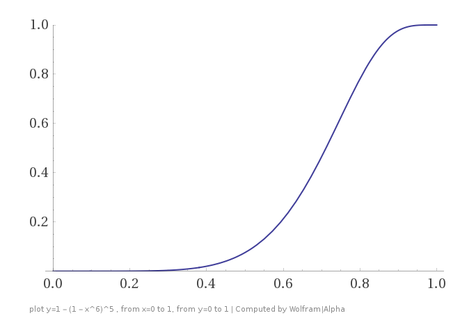
Now we can be pretty sure that things that are similar to each other will share at least one key, and things that aren’t won’t. We can increase the sharpness of the sigmoid as much as we want by spending more storage and CPU to increase A and O.
Great! Clustering with a key-value store! Now let’s talk about ways to improve
template<T>
unsigned long long int MinHash(T X, int s) {
  unsigned long long int min_hash = ULLONG_MAX;
  for (auto x : X) {
    // Note that the hash function must now accept a seed.
     min_hash = min(min_hash, Hash(x, s));
  }
  return min_hash;
}

template<T>
void EmitWithKeys(T X, int ands, int ors) {
  for (int o = 0; o < ors; o++) {
    unsigned long long int key = 0;
    for (int a = 0; a < ands; a++) {
      // we assume that a large int is enough keyspace that we
      // can get away with adding instead of concatenating.
      key += MinHash(X, a + o * ands);
    }
    Emit(key, X);
  }
}
Integer Weights
This algorithm works on a set, but the things we’d like to cluster usually aren’t sets. For instance, terms in a document (even long n-grams) can occur multiple times and ideally we don’t just want to just discard counts of how often they occur. How can we fix this?
Easy! Just hash everything multiple times. If an element occurs 
We expand our hash function to accept both an item and an integer as its argument, 


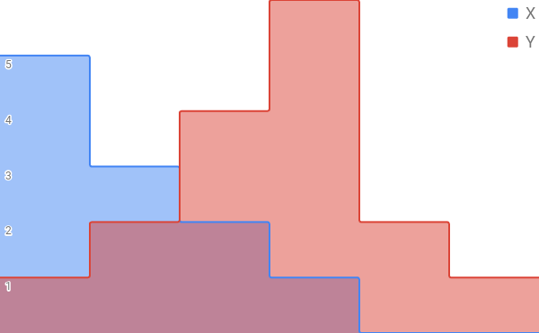
And then when you perform the intersection and union operations, these translate into performing a min and max across the values of each item.
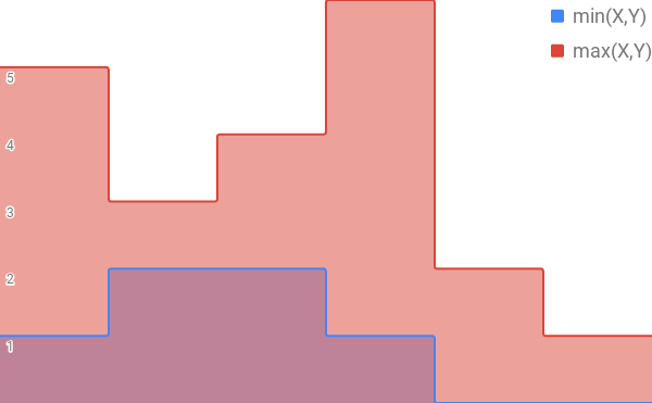
So now that we’re working with vectors instead of sets, if you interpret the Jaccard Index on this expanded set in terms of a weighted vector, it turns into the “Weighted Jaccard Index.”

template<T>
unsigned long long int IntegerWeightMinHash(map<T, int> X, int s) {
  unsigned long long int min_hash = ULLONG_MAX;
  for (auto x : X) {
    for (int i = 0; i < x.second; ++i) {
      min_hash = min(min_hash, Hash(x.first, i));
    }
  }
  return min_hash;
}
If you’d like to have 
Real Weights and Probability Distributions
Instead of going deep into the algorithms for 


The probability that the hashes collide is the “probability jaccard index” which generalizes the Jaccard index to probability distributions. (For a derivation, see our paper on minhashing probability distributions.)
![\displaystyle \Pr\left[H(x) = H(y)\right] = \sum_{i} \frac{1}{\sum_{j} \max\left(\frac{x_j}{x_i}, \frac{y_j}{y_i}\right)} = \text{J}_\mathcal{P}(x,y)](https://s0.wp.com/latex.php?latex=%5Cdisplaystyle+%5CPr%5Cleft%5BH%28x%29+%3D+H%28y%29%5Cright%5D+%3D+%5Csum_%7Bi%7D+%5Cfrac%7B1%7D%7B%5Csum_%7Bj%7D+%5Cmax%5Cleft%28%5Cfrac%7Bx_j%7D%7Bx_i%7D%2C+%5Cfrac%7By_j%7D%7By_i%7D%5Cright%29%7D+%3D+%5Ctext%7BJ%7D_%5Cmathcal%7BP%7D%28x%2Cy%29&bg=%23ffffff&fg=%23000000&s=0&c=20201002)
This is a strange looking formula, what is it? And why is it the Jaccard Index of probability distributions? We’ll get to that in the next section. First, let’s figure out why this particular transformation works. It has to do with the beautiful things exponential random variables do when you sort them.
A variable ![\Pr\left[X<y\right] = 1 - e ^{-\lambda y}](https://s0.wp.com/latex.php?latex=%5CPr%5Cleft%5BX%3Cy%5Cright%5D+%3D+1+-+e+%5E%7B-%5Clambda+y%7D&bg=%23ffffff&fg=%23000000&s=0&c=20201002)

The distribution of the minimum of two random variables is easy to derive from their distributions. ![\Pr\left[\min(X_1,X_2) < y \right] = \Pr\left[X_1 > y\right]\Pr\left[X_2 >y \right]](https://s0.wp.com/latex.php?latex=%5CPr%5Cleft%5B%5Cmin%28X_1%2CX_2%29+%3C+y+%5Cright%5D+%3D%C2%A0%5CPr%5Cleft%5BX_1+%3E+y%5Cright%5D%5CPr%5Cleft%5BX_2+%3Ey+%5Cright%5D&bg=%23ffffff&fg=%23000000&s=0&c=20201002)


![\Pr\left[\min(X_1,X_2) < y \right] = 1 - e ^{-(\lambda_1 + \lambda_2) y}](https://s0.wp.com/latex.php?latex=%5CPr%5Cleft%5B%5Cmin%28X_1%2CX_2%29+%3C+y+%5Cright%5D+%3D%C2%A01+-+e+%5E%7B-%28%5Clambda_1+%2B+%5Clambda_2%29+y%7D&bg=%23ffffff&fg=%23000000&s=0&c=20201002)


![\displaystyle\Pr\left[X_1 = \min(X_1, X_2)\right]](https://s0.wp.com/latex.php?latex=%5Cdisplaystyle%5CPr%5Cleft%5BX_1+%3D+%5Cmin%28X_1%2C+X_2%29%5Cright%5D&bg=%23ffffff&fg=%23000000&s=0&c=20201002)
![\displaystyle\int_{y=0}^\infty \Pr\left[X_1 \in (y, y+dy)\right]\Pr\left[X_2>y\right] dy](https://s0.wp.com/latex.php?latex=%5Cdisplaystyle%5Cint_%7By%3D0%7D%5E%5Cinfty+%5CPr%5Cleft%5BX_1+%5Cin+%28y%2C+y%2Bdy%29%5Cright%5D%5CPr%5Cleft%5BX_2%3Ey%5Cright%5D+dy&bg=%23ffffff&fg=%23000000&s=0&c=20201002)
![\displaystyle\int_{y=0}^\infty\Pr\left[X_1 \in (y, y+dy)\right]\left(1 -\Pr\left[X_2<y\right] \right) dy](https://s0.wp.com/latex.php?latex=%5Cdisplaystyle%5Cint_%7By%3D0%7D%5E%5Cinfty%5CPr%5Cleft%5BX_1+%5Cin+%28y%2C+y%2Bdy%29%5Cright%5D%5Cleft%281+-%5CPr%5Cleft%5BX_2%3Cy%5Cright%5D+%5Cright%29+dy&bg=%23ffffff&fg=%23000000&s=0&c=20201002)


This gives us a new way of sampling from a distribution. If I have a probability distribution with parameters 
So, back to minhashing. Instead of generating exponential random variables, now we want to generate “exponentially distributed hashes.” To do that, all you have to do is take a uniformly distributed hash from 0 to 1, invert the exponential CDF, and apply it.
Then if we take the minimum of all these exponentially distributed hashes, we have a sample from the distribution that is stable under small changes, just like the original MinHash!
template<T>
T ProbabilityMinHash(map<T, float> X, int s) {
  pair<double, T> min_hash;
  min_hash.first = std::numeric_limits::infinity;
  double maximum_hash = ULLONG_MAX;
  for (auto x : X) {
    double zero_one_hash = Hash(x.first) / maximum_hash;
    pair<double, T> exponential_hash(-log(zero_one_hash) / x.second, x.first);
    min_hash = min(exponential_hash, min_hash);
  }
  return min_hash.second;
}
Understanding the Probability Jaccard Index
How do you compute the “union” of two probability distributions? How do you compute an “intersection?” One proposal might be to use the 


 can be thought of as rescaling the two distributions before computing each term of so that the in the numerator has no effect.
How can we fix this? We’d like to normalize the distributions in some way so that this no longer happens. Our goal is to make it so that uniform distributions have the same likelihood of colliding as when we applied MinHash to the set that they’re distributed over. Let’s generalize 

Now, since 


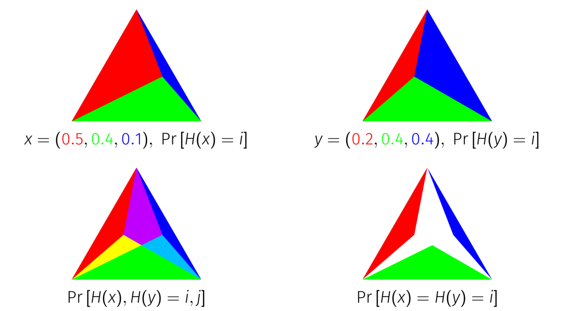
 You can derive another representation using the algorithm definition. A set of exponential random variables, when normalized to sum to 1, is a uniformly distributed sample from the unit-simplex. (A unit-simplex is an equilateral triangle in n-dimensions.) In addition, because a unit-simplex is just the set of non-negative vectors that sum to 1, every point on the unit simplex is a probability distribution.
From this, we can represent
Take the unit simplex and mark the point on the simplex that corresponds to the distribution you would like to hash. Connect that point to each corner of the simplex with an edge. These edges you’ve drawn split the simplex into smaller simplexes, where each one has area proportional to the weight of one of the elements of your distribution.
With the distribution represented this way, you can imagine sampling from it by throwing darts at the simplex. The id of whichever region the dart lands in is a sample from your distribution. The probability MinHash does exactly this, except that the dart remains in the same spot for each distribution you sample from, and the boundaries of the regions shift around it.
 geometrically as an intersection of simplexes.
So now, we’re able to visualize
This representation also lets us demonstrate geometrically the most interesting fact about
Theorem:
For any sampling method, if
, then for some
where
and
, either
or
.
In other words, no method of sampling from discrete distributions can have collision probabilities that are greater than
This theorem is true of 


The proof of this in the general case is complicated, but the simplex representation allows us to prove it purely visually on three element distributions.
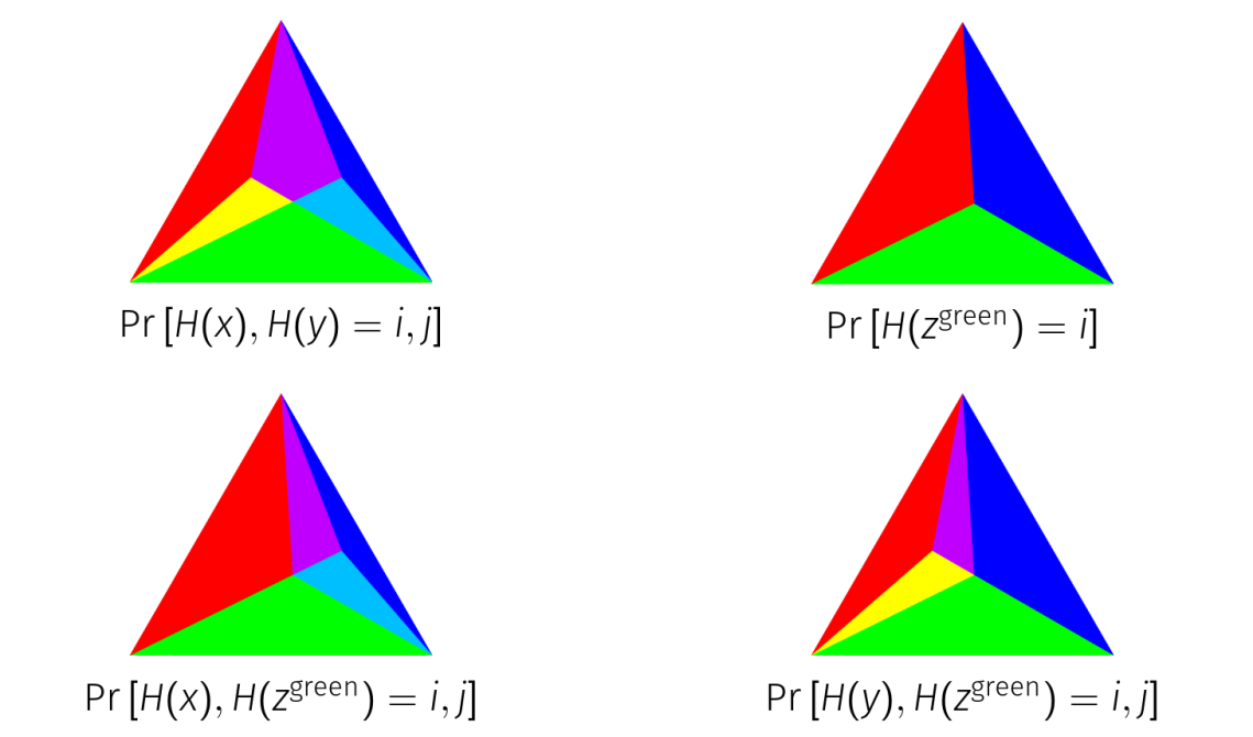 and could be shifted to overlap more, but doing so would remove collisions between both of them and
  .
.We form a new distribution out of the intersection of the green simplexes. This makes a distribution that is in-between
For a lot more about this see our Probability Minhash paper.
